Previous lab. Return home. Next lab.
In lecture, I had previously connected the IMU to the Artemis via the QWIIC cable.
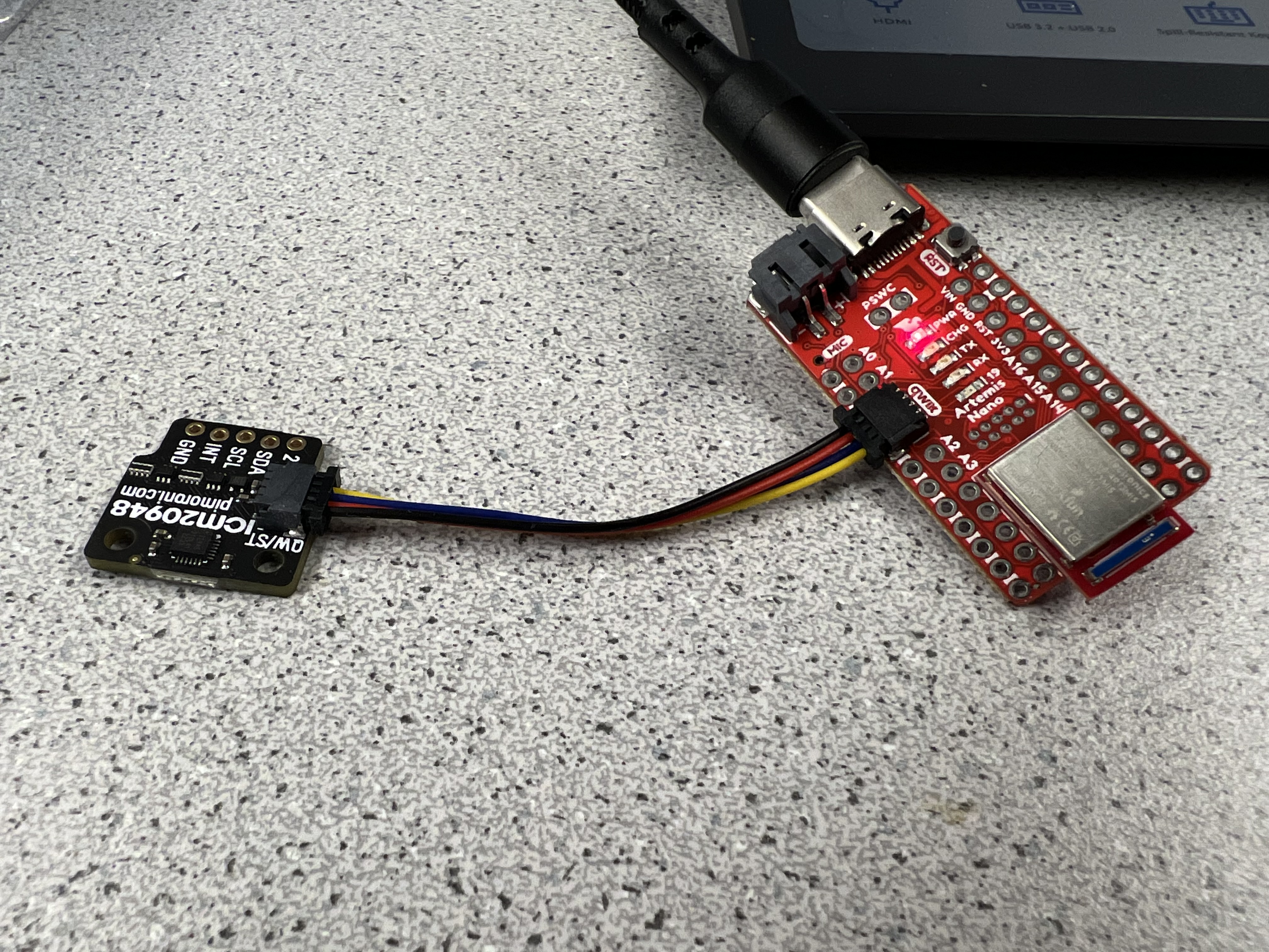
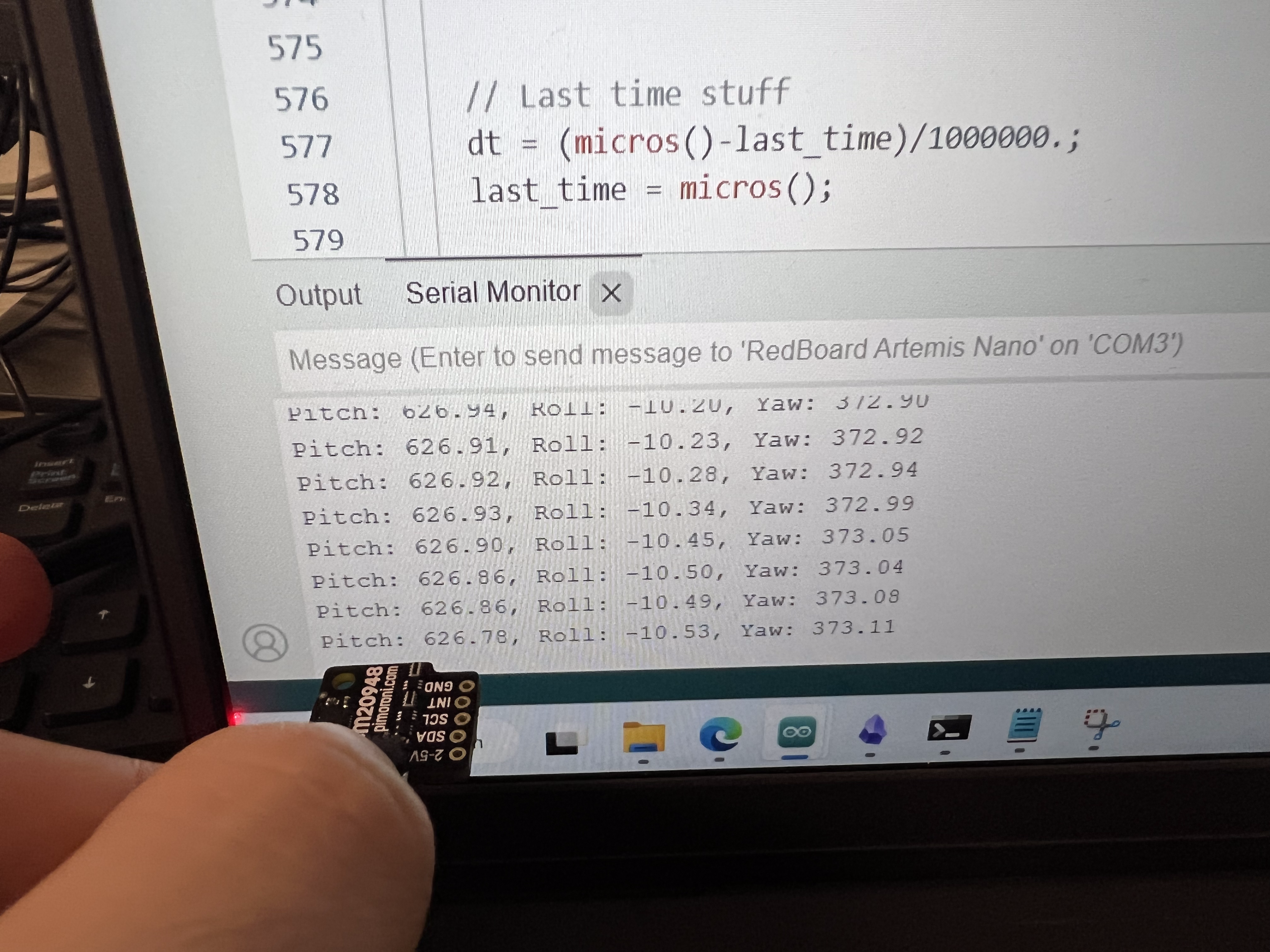
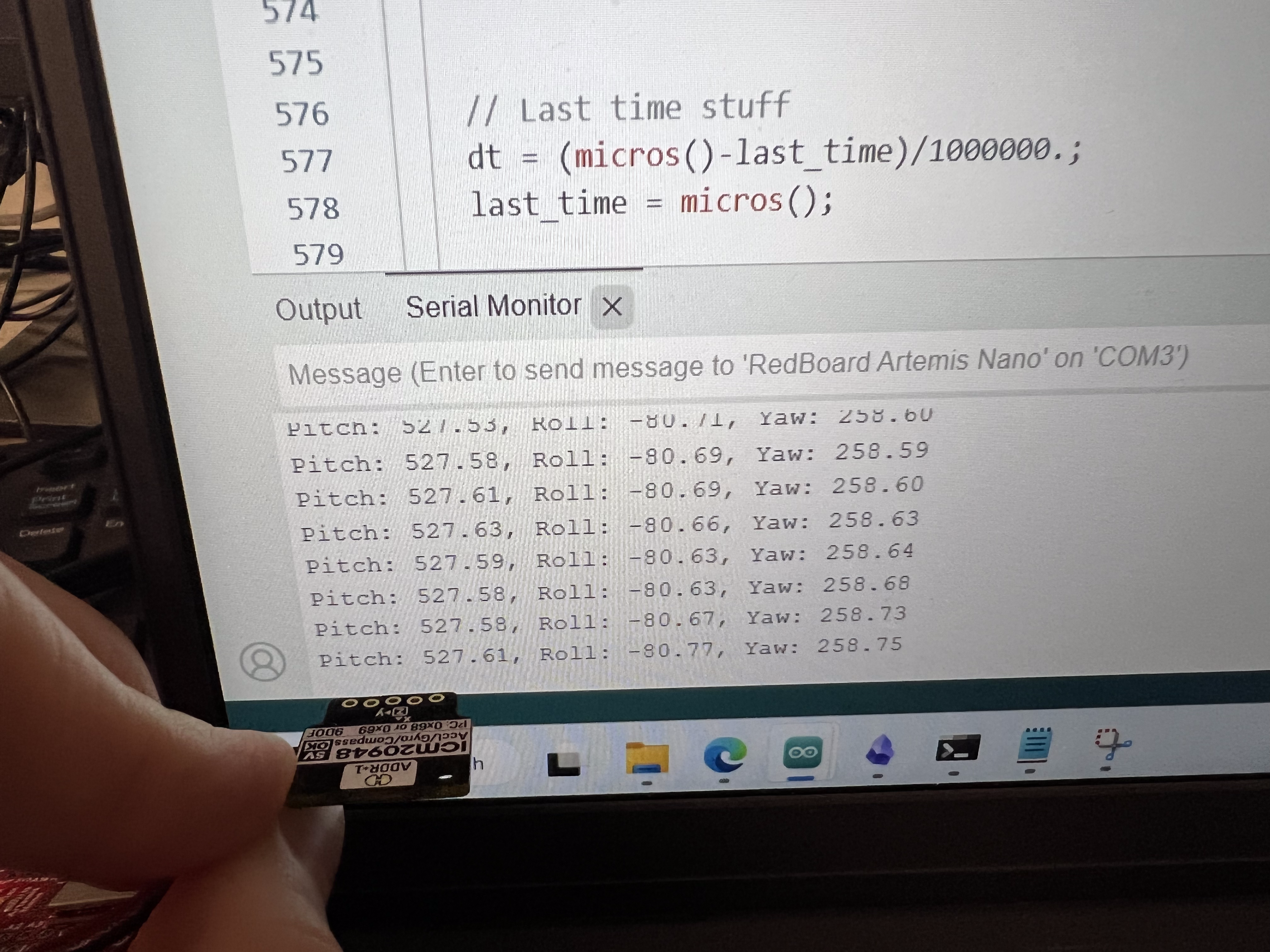
For my IMU to work, I had to set AD0_VAL to 0 instead of the default 1. AD0_VAL is the value of the last bit of the I2C address, which is used for communication between the IMU and the Artemis. Because this has to be 0 for my IMU to work, the I2C address of my IMU is 0x68 and not 0x69. Once this was done, the IMU demo code worked (see below the Serial output).
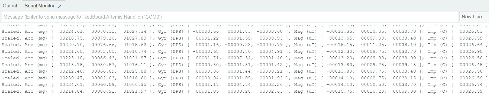
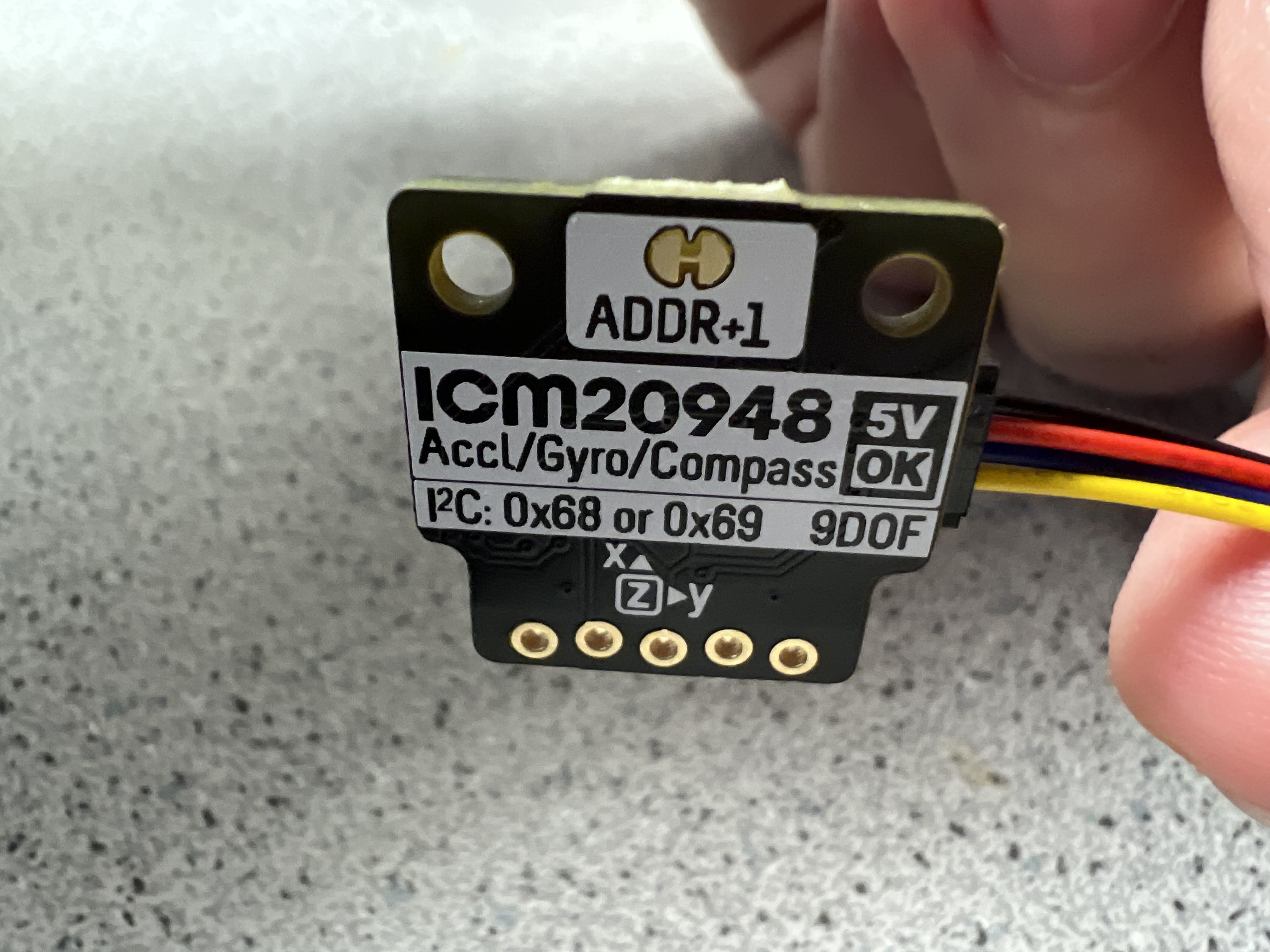
When rotating the board around the board's x axis, the accelerometer data for y and z change, while the gyroscope data for x changes. When rotating the board around the board's y axis, the accelerometer data for x and z change, while the gyroscope data for y changes. When rotating the board around the board's z axis, the accelerometer data does not change, but the gyroscope data for z does. Below is an image of the axes printed on the chip.
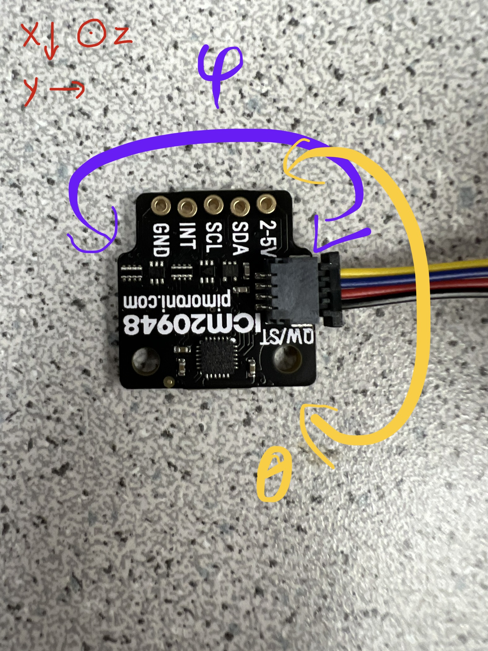
The next image represents the rotations that change the accelerometer data. The top left arrows shows the orientation of the axes. The rotation arrow on the top shows rotation around the x axis, or roll. The rotation arrow on the right shows rotation around the y axis, or pitch.
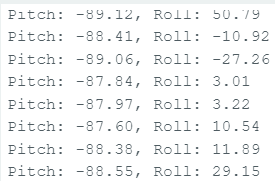
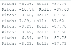
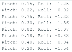
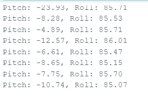
The next step is to use this to calculate the pitch and roll with respect to the axes of the IMU. The table below shows the pictures of the Serial output of the following orientations.
| Pitch: -90, Roll: 0 | Pitch: 0, Roll: -90 | Pitch: 0, Roll: 0 | Pitch: 0, Roll: 90 | Pitch: 90, Roll: 0 |
|---|---|---|---|---|
|
|
|
|
|
I used the following to get the pitch and roll:
pitch_a = atan2( ICM.accX(), ICM.accZ() ) * 180/M_PI;
roll_a = atan2( ICM.accY(), ICM.accZ() ) * 180/M_PI;
My accelerometer isn't very accurate. When one measurement is at 90 degrees, the other measurement is quite jittery. Only when they are both around 0 is it more stable, but even then, it still isn't quite accurate. I could have attempted to adjust using a two-point calibration, but I honestly think that once I get a filter on these values, they will be much more accurate, even if off by only a few degrees.
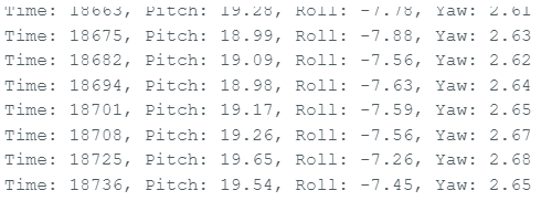
To guide my choices regarding my complimentary lowpass filter for the accelerometer data, I needed to actually gather some data. I needed to figure out what kind of noise my robot would be producing that would interfere with this data. To start off, I needed to create a system for gathering and sending the data from the IMU to the computer for further analysis. This was relatively straightforward, given that something like it had already been done in the previous lab.
// If we want to gather IMU data
if( get_IMU_data ) {
// But the IMU data is full
if( IMU_entries_gathered >= IMU_ARRAY_SIZE ) {
// Set that we don't want to send IMU data anymore
get_IMU_data = false;
// Set that we want to send our data
send_IMU_data = true;
}
// If that previous condition was true (too much data), then it will skip this else.
// If that previous condition was false (still room), then if the data is ready, this will execute collecting data.
else if( ICM.dataReady() ) {
// The values are only updated when you call 'getAGMT'
ICM.getAGMT();
// Gather the data into their respective arrays
time_array[IMU_entries_gathered] = (int) millis();
pitch_array[IMU_entries_gathered] = atan2( ICM.accX(), ICM.accZ() ) * 180/M_PI;
roll_array[IMU_entries_gathered] = atan2( ICM.accY(), ICM.accZ() ) * 180/M_PI;
// Increment the counter
IMU_entries_gathered++;
}
}
And...
// Whether or not we want to gather IMU data, if we want to send it, we will send it.
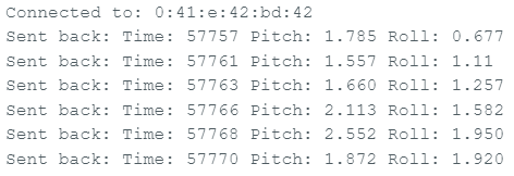
if( send_IMU_data ) {
for( int i = 0; i < IMU_entries_gathered; i++ ) {
tx_estring_value.clear();
tx_estring_value.append( "Time: " );
tx_estring_value.append( time_array[i] );
tx_estring_value.append( " Pitch: " );
tx_estring_value.append( pitch_array[i] );
tx_estring_value.append( " Roll: " );
tx_estring_value.append( roll_array[i] );
tx_characteristic_string.writeValue( tx_estring_value.c_str() );
Serial.print( "Sent back: " );
Serial.println( tx_estring_value.c_str() );
}
// We don't want to get stuck in a horrible Bluetooth loop
send_IMU_data = false;
// When we are done sending the data, we need to essentially wipe the array clean by just resetting the index, or the IMU_entries_gathered
IMU_entries_gathered = 0;
}
The code to collect is done in the write_data() function, so as to allow the data to be gathered at the speed of the main loop, and only when we want to, as it is ignored if get_IMU_data is false. The code to send is done in the read_data() function, and it is also ignored unless we are explicitly trying to send data. The flag get_IMU_data is set by the command GET_ACCELEROMETER_DATA, and the flag send_IMU_data can also be set by the command SEND_ACCELEROMETER_DATA. However, I found I never used that command and just waited for the IMU array filling mechanism to flip that flag for me.
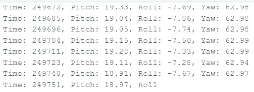
Once we have gathered and sent the IMU data to the computer, we now need to run an FFT on it. We collected time data, so as to allow us to see the accelerometer data versus time, along with the pitch and roll. The code segment below shows how the Python FFT was performed on the data, where pitch_y and roll_y are the Fourier data of the pitch and roll respectively.
samples = len( time )
freq_data_pitch = fft( pitch )
freq_data_roll = fft( roll )
pitch_y = 2/samples * np.abs( freq_data_pitch[0:np.uint64( samples / 2 )] )
roll_y = 2/samples * np.abs( freq_data_roll[0:np.uint64( samples / 2 )] )
This yields the following graphs.
.png) |
.png) |
.png) |
|
Now, with the robot on, these were the resulting graphs.
.png) |
.png) |
.png) |
|
Admittedly, I believe this increase in noise was likely due to my shaking the IMU much more than any robot interference. There doesn't seem to be much more in the way of high-frequency noise, though I am sure a low-pass filter would still smooth things out and make the readings more workable. While there is noise in the graphs all the way to the lowest frequencies, it might be good to choose a lower frequency for the cutoff to start off to remove a reasonable amount of the noise.
It is also important to consider the sampling rate of the IMU. Over the course of 3979 milliseconds, it collected 1024 samples. This is about 257 samples per second. Thinking back to the Nyquist-Shannon sampling theorem, we will pick up on meaningful noise below 128.5 Hz, meaning that our filter should be a reasonable amount lower than that. Perhaps on the order of 50 or so Hz for the cutoff frequency might be a good place to start.
Using this, I implemented a low-pass filter. I used a cutoff frequency of 50 Hz, meaning an RC constant of 0.003183. I assumed 257 samples per second, meaning a T of 0.003891. Using these, alpha was calculated to be about 0.55. In my implementation, I found it easier just to use roll as the pitch's low-pass output instead of programming a lot more in the way of new arrays for data and transmitting all of that data.
roll_array[IMU_entries_gathered] = alpha * pitch_array[IMU_entries_gathered] + ( 1 - alpha ) * ( IMU_entries_gathered == 0 ? 0 : roll_array[IMU_entries_gathered - 1] );
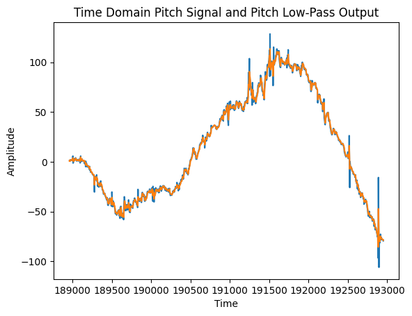
The blue graph is the unfiltered pitch, while the orange graph is the low-pass output for the pitch. It definitely does help those big spikes, but it is not much smoother. Perhaps a cutoff frequency of 25 might smooth it out more.
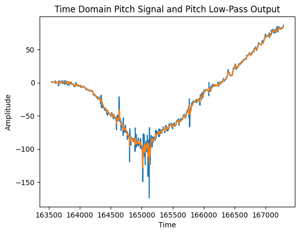
It does seem to be a bit smoother at an alpha of 0.38, and I'm sure this could be taken even further, need be.
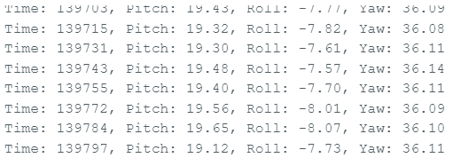
Well, perhaps the first thing to note is that we can actually get a value for yaw with the gyroscope, whereas with the accelerometer, we could not. The same thing goes for the filtered accelerometer data. There simply was no yaw value.
One very noticable difference as well is that at the 90 degree angle for one measurement, the other measurements are quite stable. This was absolutely not the case with pitch and roll with the accelerometer, where the slightest change brought it from -90 to 90, and anywhere in between was incredibly jittery. And that was also the case with the filtered accelerometer readings.
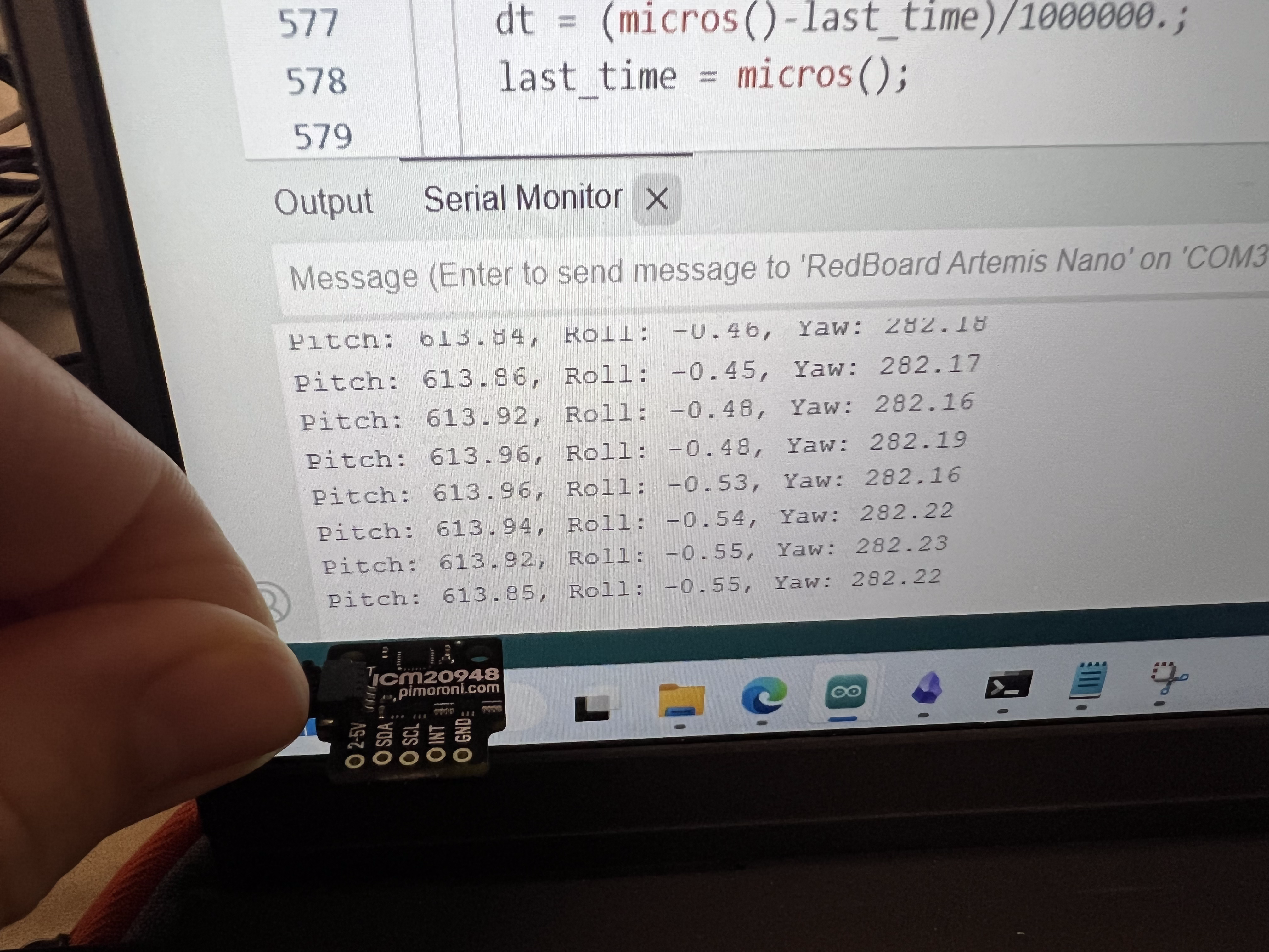
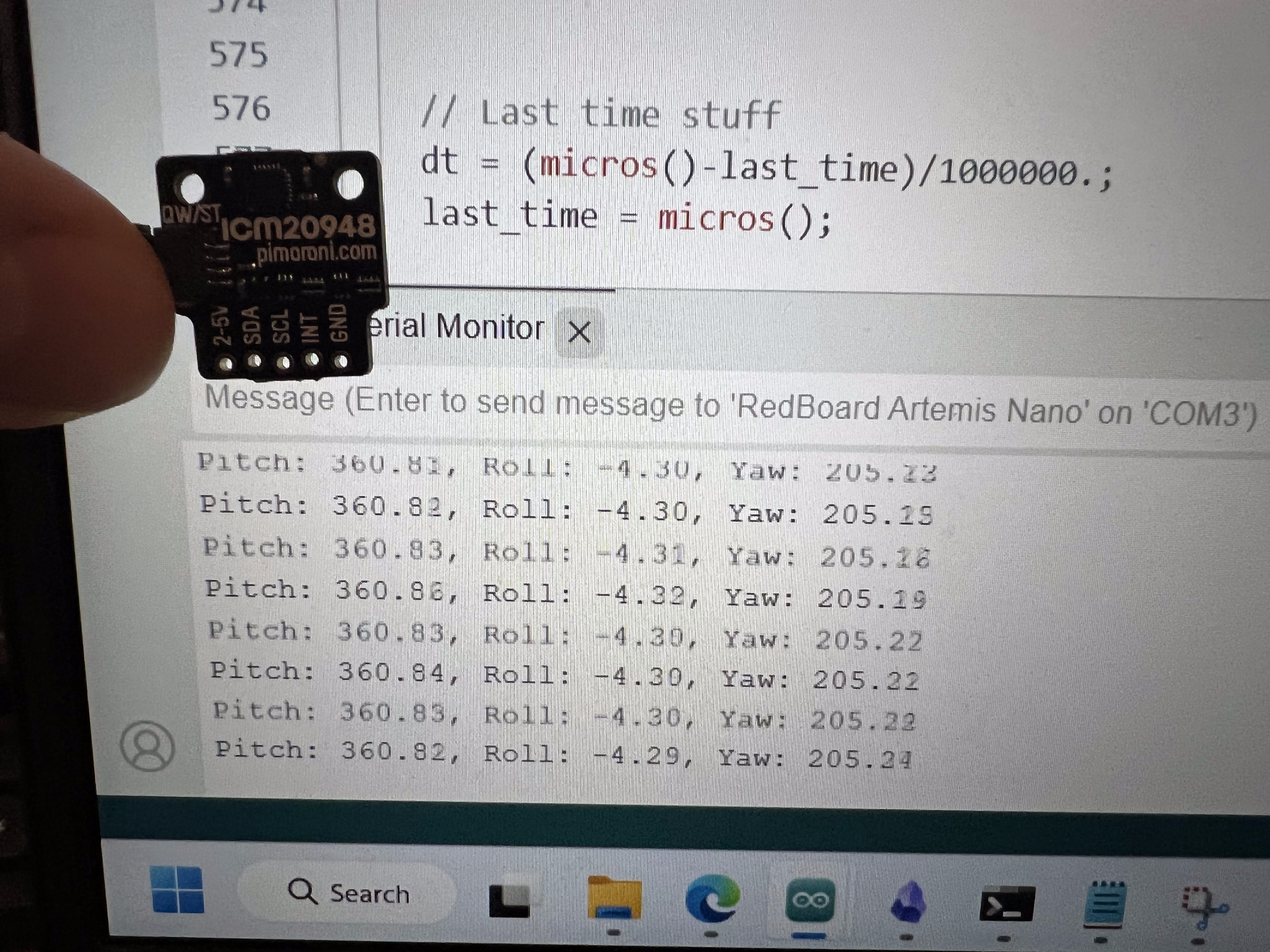
Another difference is that the calculated positions are not absolute, as they were with the accelerometer. It varies based on the speed of rotation and previous positions. This can make for some difficulties. This is also related to the drift, which occurs over time and will slowly approach a steady-state value for the measurements if the IMU is left alone. This ultimately means it can take some pretty strange values over time.
 |
 |
 |
 |
For the complimentary filter, it seems much more stable. Leaving the IMU on the table, it rarely jitters beyond one degree of error. By weighing the accelerometer data equal to the gyroscopic data (alpha = 0.5), the drift from the gyroscope has an even lesser effect than it previously did. Leaving The gyroscope alone for well over two minutes did not change the value of pitch or roll visibly at all. Meanwhile, the change in yaw from drift is very clear.
 |
| |  |
| |  |
In terms of speeding up the main loop, I basically had done that already in order to collect the data for the accelerometer. There is no waiting for the IMU, no delays, and no Serial.print() statements in the sampling code. I previously had found my board could sample at around 257 Hz. My main loop is only a little faster than this, running at around 276 Hz, as it collected 1024 samples in 3711 milliseconds.
Once again, I already collected the IMU data in arrays using flags in the main loop. The code snippets for this can be seen in the accelerometer section.
In terms of data storage, I opted for separate arrays to store my data. The individual lengths of the arrays can be adjusted to correspond to the relative frequency at which the data can be sampled. Also, in my mind, it is easier to work with separate arrays than one giant array. You can have different data types for each array instead of being forced into one data type for one large array.
In terms of the data type, it depends, but strings should generally be avoided when storing numbers. They use one byte per character, and for an integer with 5 digits, it would take 5 bytes, whereas a 5 digit integer, if less than 65536, could be stored in two bytes, which is much more memory dense! If great precision is needed, doubles are a good idea, but they are quite large in memory usage, so they should be used sparingly. Most of the time, floats should be sufficient for decimal values.
In terms of the amount of memory the Artemis has for variables, it seems to be 393216 bytes, according to the output of the Arduino IDE console. Assuming we're only storing 32-bit integers, or 4-byte integers, that gives us an array of length 98304 samples with which to work. Assuming 257 samples per second, this should give us about 382 seconds total, with only about 1285 samples being needed to record the five minutes requested.

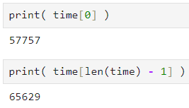
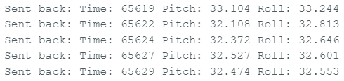
The time of the recorded data ranges from 57757 milliseconds to 65629 milliseconds. This represents a time difference of 7872 milliseconds, or 7.872 seconds.
 |
 |
 |
As is perhaps evident in the video, the car moves very quickly and is quite difficult to control precisely. I am curious how much that will carry over to how easily the robot will be able to be controlled with precision as we progress through the semester.
I unfortunately did not get to record a video of the stunt car with the Arduino, as that would have required soldering and getting the Artemis powered separately from my computer. I'd imagine, though, that Artemis would be able to collect some data that could be useful for learning what data might need to look like in future labs when certain stunts are being performed, when I am not controlling the robot with the remote.