Previous lab. Return home. Next lab.
In this lab, we will be working with the VL53L1X Time of Flight (ToF) sensor. According to the datasheet, it has an I2C address of 0x52 when the ToF sensor reads from the Artemis, and 0x53 for when the Artemis is receiving data. We have two of these ToF sensors with the same I2C address. The address can be changed. However, both sensors will be connected listening, so we need a way to just change one and not the other. The VL53L1X has a pin called XSHUT (Xshutdown), which when low, the chip enters hardware standby mode, which is important in terms of disabling I2C communication. This should allow us to change the address of one without changing the address of the other, preventing address collisions when we want to communicate with them.
Though it is possible to just communicate with one at a time by disabling the other, I think it will be easier to coordinate communication with both devices by just changing the address of one of them, instead of maintaining that only one sensor be not in hardware standby at any time.
To start to consider where I will place the sensors on my robot, it is important to consider what kind of Field of View (FOV) the sensors have. The datasheet states the assumption that the ToF sensors typically have a FOV of about 27 degrees. So one thing to consider would be placing the sensors where they won't be blocked. On the sides of the car, between the wheels, for example, does not seem like not a viable option. One obvious location would be the front or back of the car. Another possible location would be the top of the car, which could prove useful if the car is doing flips. However, I don't think it would realistically be worth it to place a sensor there, as it would almost always be pointing at the ground or at the sky. Putting both on the front would not be quite useful, as the car will often be moving backwards, and it would be doing so blindly. I, am led to believe the best would then be one in the front and one in the back.
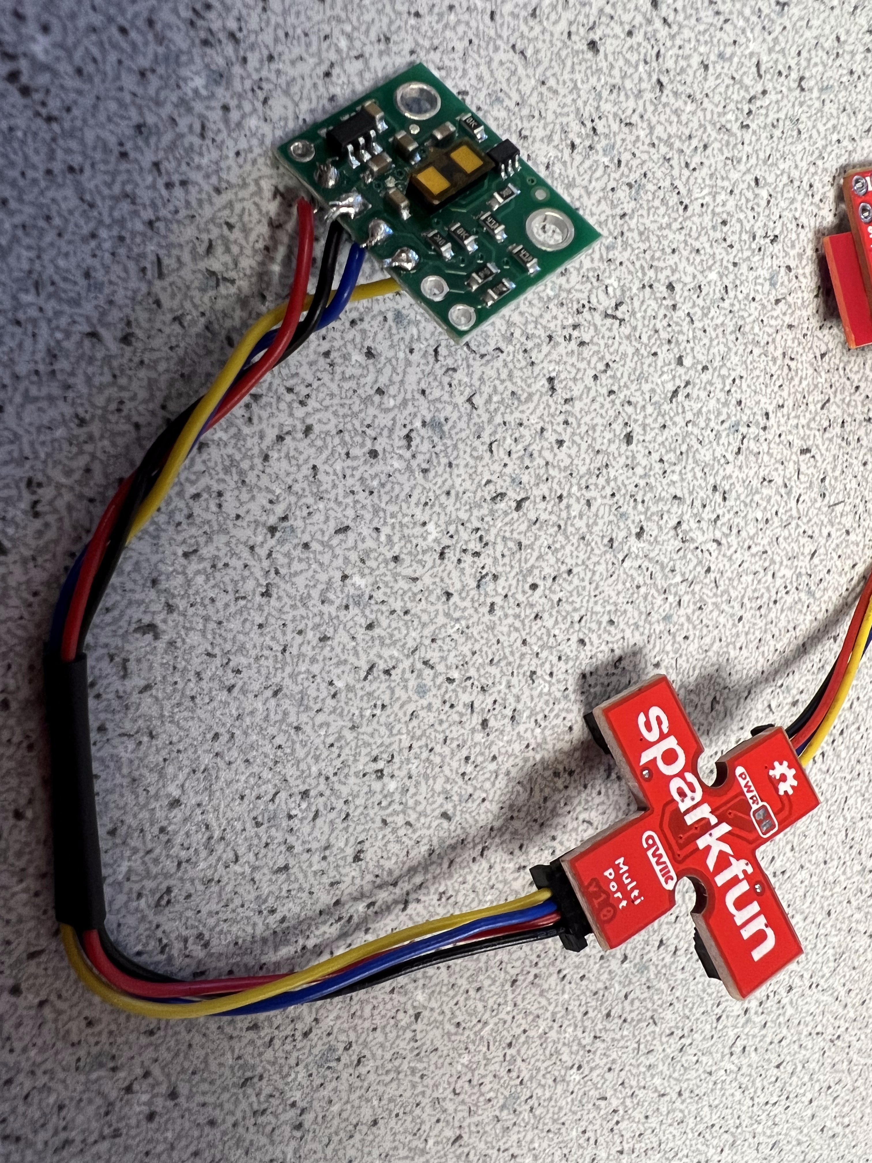
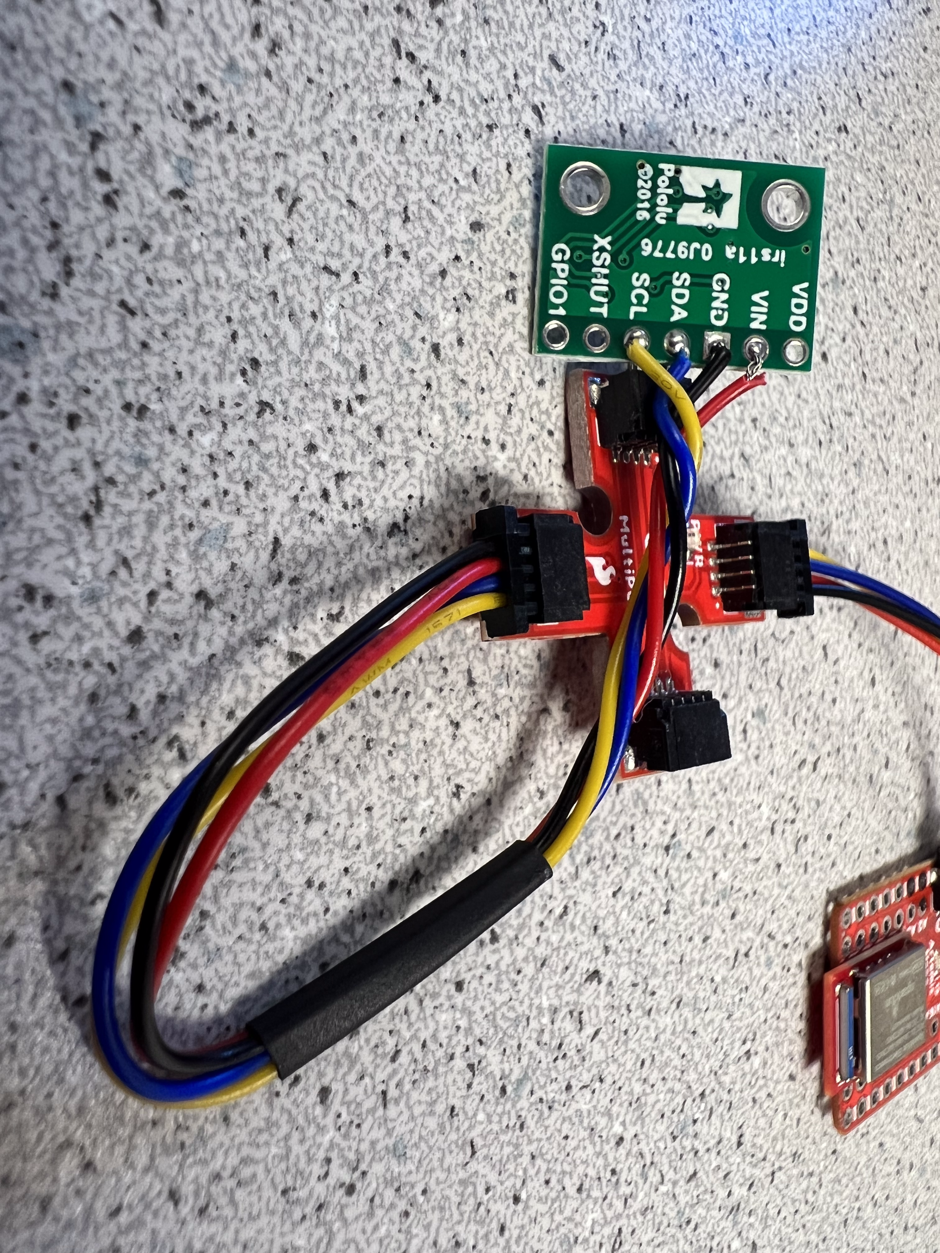
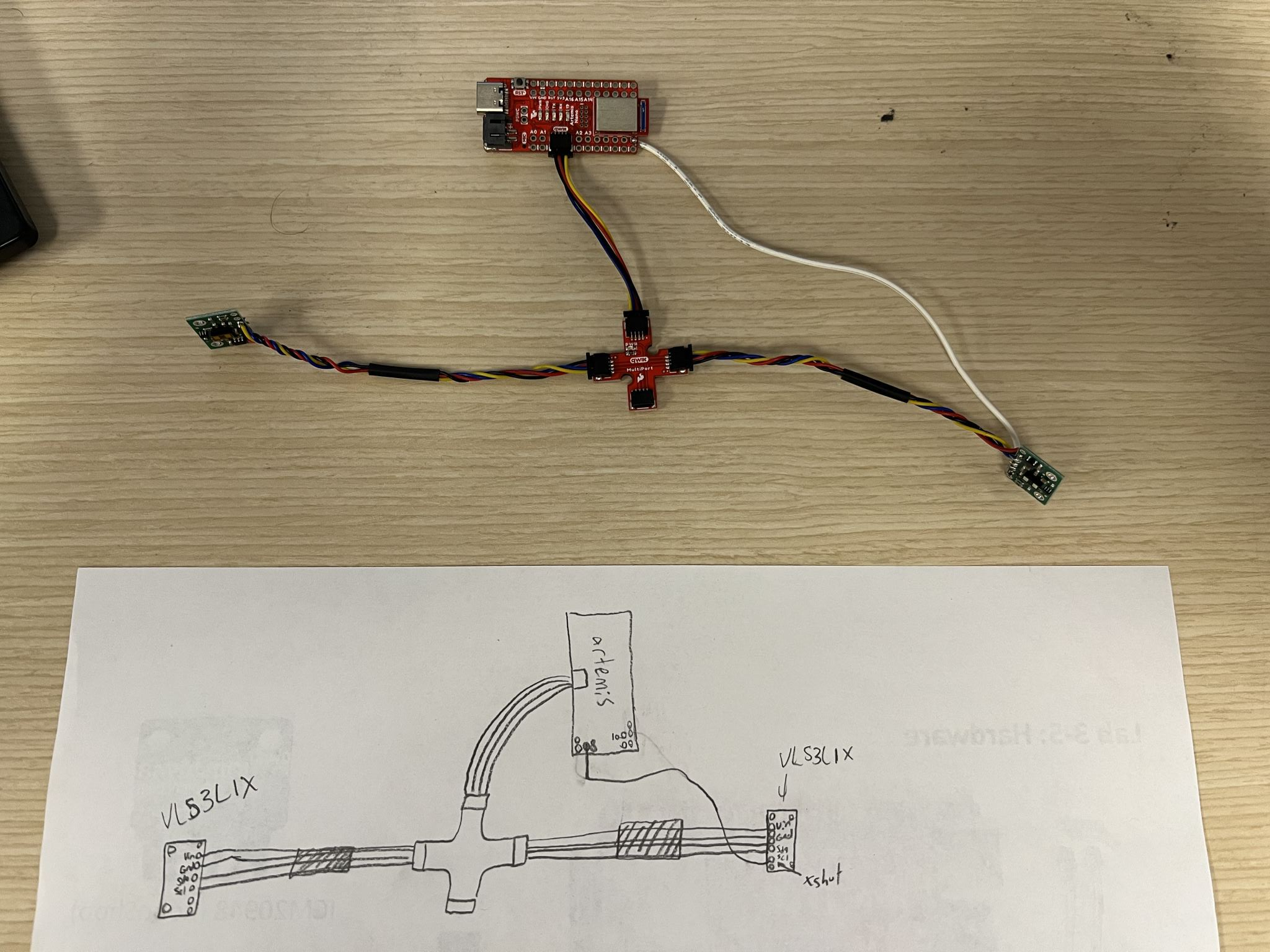
Below is my wiring diagram, alongside what I actually assembled.
|
|
|
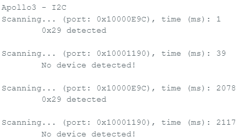
The address that was displayed was 0x29. This address translates to 0010 1001 in binary. When looking at the documentation, as I mentioned earlier, the ToF sensor is supposed to have an address of 0x52, which translates to 0101 0010 in binary. This is the displayed address shifted to the left by 1. This is because the last R/W bit goes unset, and therefore isn't read.
Looking at the datasheet for the different distance modes, the advantage of the short distance mode is that it is more resilient against noise. The advantage of the long distance mode is that it generally has the longest range, but the least resilience against noise. At long distance and strong ambient light, it actually has the least distance. The environments in which this car will drive will likely be in relatively bright environments, which makes me wonder if the short distance mode is a viable option to consider long-term. Whatever the long-term option may be, for now, I will opt to work with the short-range, as it is most resilient to noise and my robot shouldn't be moving fast enough to need a longer-range.
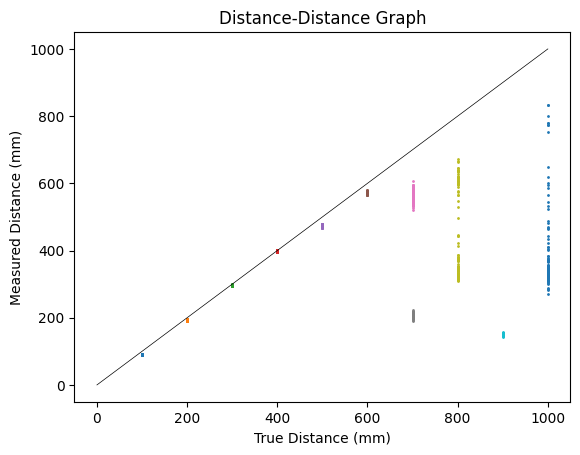
I planned to measure values from 100 millimeter up to 1000 millimeters, at increments of 100 millimeters. At each of these increments, I took 100 samples. Toward the start, the sensor was fairly reliable. Toward the end, however, the sensor started to become less and less reliable. At 700 millimeters, I shut off the lights for a second round of samples because the measurements were starting to get bad. This made the sampling even worse. From there it dropped off. At the end, I did another test with 100 millimeters to make sure the sensor wasn't broken during testing, however, the readings were pretty consistent with the first set of readings at 100 millimeters, so I left them out of the graph. To construct the graph, I just plotted each data point against the expected data point. This creates what will be columns centered around each 100-millimeter increment. This creates a nice visualization of the spread of the data at each increment.
In terms of sensor speed, I took 2048 samples twice. The first sample set's time ranged from 527837 to 629599, with a range of 101762. The second's ranged from 885091 to 986846, with a range of 101755. These are pretty consistent with each other, so I will just average the value out, and use that to calculate the sensor rate. With a rate of 2048 samples in 101.7585 seconds, that comes out to about 20.126 samples per second, or about 49.687 milliseconds per sample.
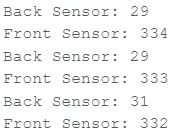
The image shown in the prelab section shows both of the sensors properly connected to the Artemis. Below is a screenshot of the serial output showing measurements from both sensors.
Below is the code that I wrote to be able to get the two sensors properly working.
// We first want to set XSHUTDOWN to low. This will disable the front sensor
digitalWrite( XSHUTDOWN, LOW );
// We first want to check if a sensor is set to 0x52. If it is, it means the back sensor is, as that is the only sensor that can respond
if( distance_sensor_back.getI2CAddress() == 0x52 ) {
// We then want to set the back sensor to 0x54 to differentiate it.
distance_sensor_back.setI2CAddress( 0x54 );
}
// If it is not 0x52, then we already set it to 0x54.
// We then want to check if it initialized well. It will return 0 if so.
if( distance_sensor_back.begin() != 0 ) {
Serial.println( "Back distance sensor failed to begin. Please check wiring." );
}
// If it did
else {
// set the distance mode
distance_sensor_back.setDistanceModeShort();
// and display that it worked.
Serial.print( "Back sensor online with distance mode " );
Serial.print( distance_sensor_back.getDistanceMode() );
Serial.print( " and at address 0x" );
Serial.println( distance_sensor_back.getI2CAddress(), HEX );
}
// Then enable the XSHUTDOWN pin so that we might enable the front sensor
digitalWrite( XSHUTDOWN, HIGH );
// Begin returns 0 on a good initialization
if( distance_sensor_front.begin() != 0 ) {
Serial.println( "Sensor failed to begin. Please check wiring." );
}
else {
// Set the distance mode
distance_sensor_front.setDistanceModeShort();
// and display that it worked.
Serial.print( "Front sensor online with distance mode " );
Serial.print( distance_sensor_front.getDistanceMode() );
Serial.print( " and at address 0x" );
Serial.println( distance_sensor_front.getI2CAddress(), HEX );
}
Using this, along with the data collection and sending code that will be outlined later in the lab (though that code has been since modified for to get the front and back sensors to send separately), I created a graph with the results of the two sensors.
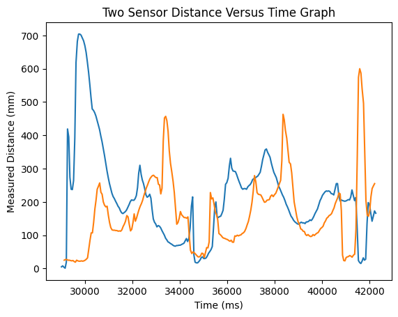
As seen in the picture above, the time between each loop iteration is, on average, a bit faster than the time between loop iterations where a distance measurement is recorded. This means that the distance measurements are likely the limiting factor, though, it seems the loop time can vary a lot and there might be times the loop itself might be the problem.
As with the previous lab, I had the Artemis gather the sensor data into an array. This time, however, because I will be gathering data from multiple sensors, I wanted the time to be more intimately connected with the data. So I used a struct with the distance and time data bundled together, and created an array of those structs. Below are the code snippets of how I did this.
// Check if the data from the sensor is ready to be collected
if( distance_sensor_front.checkForDataReady() ) {
// Get the time as early as possible so it is most accurate to when data was gotten
distance_array[distance_entries_gathered].time = (int) millis();
// Get the result of the measurement from the sensor
distance_array[distance_entries_gathered].distance = distance_sensor_front.getDistance();
// Stop ranging and set ranging to false
distance_sensor_front.clearInterrupt();
distance_sensor_front.stopRanging();
ranging = false;
// Increment our entries gathered variable.
distance_entries_gathered++;
}
And...
// Whether or not we want to gather distance data, if we want to send it, we will send it.
if( send_distance_data ) {
for( int i = 0; i < distance_entries_gathered; i++ ) {
tx_estring_value.clear();
tx_estring_value.append( "Distance: " );
tx_estring_value.append( distance_array[i].distance );
tx_estring_value.append( " Time: " );
tx_estring_value.append( distance_array[i].time );
tx_characteristic_string.writeValue( tx_estring_value.c_str() );
Serial.println( tx_estring_value.c_str() );
}
// We don't want to get stuck in a horrible Bluetooth loop
send_distance_data = false;
// When we are done sending the data, we need to essentially wipe the array clean by just resetting the index, or the IMU_entries_gathered
distance_entries_gathered = 0;
}
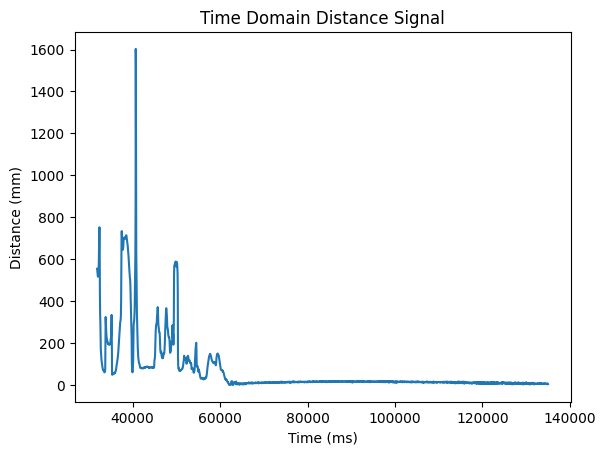
Processing the data produced by this in the Jupyter Notebook allowed me to produce this plot. I moved the sensor around a lot at the start before putting it down, as it was taking longer than I expected it to.
There are a variety of infrared-based sensors. A passive infrared sensor senses the infrared radiation emitted from an object. This is useful for detecting the presence of a being that emits infrared light, or heat. This is useful in applications involving passive lighting (bathrooms at Cornell where the lights turn on when you walk in) or even security applications (cameras activate when they detect heat). These aren't so useful when you want to detect any object. These also aren't really able to detect distance. To do that, an active infrared sensor that emits infrared light and detects its return is needed. This has its applications in things like robotics (this course, where we can tell the distance of an obstacle). However, this kind of sensor must actively emit infrared raditation to find the distance. Other sources of infrared radiation might be able to interfere and decrease the accuracy of this sensor. Other types of sensors are things such as infrared cameras which are used to produce images of the world by detecting infrared light and infrared temperature sensors which can characterize the temperature of an object by sensing the infrared raditation of the object.
Thanks to this page for the helpful rundown of infrared-based sensors! (external link) https://www.electronicsforu.com/technology-trends/learn-electronics/ir-led-infrared-sensor-basics.
At a range of 300 millimeters, the texture nor color don't seem to affect the readings much. I used a black fabric, a white fabric, a light blue fabric, a black glossy cardboard, a white glossy cardboard, and a light blue glossy cardboard, and none of them seemed to differ very much. If anything, the white glossy surface was measuring about 10 millimeters under 300, while the others seemed to mostly average 300 millimeters.