Previous lab. Return home. Next lab.
Sigma_z is just the variance of the sensor reading. The sensor I am using is the front distance sensor. We can see that the front distance sensor's variance is a function of the distance. Calling back to lab 3, we can see the spread of the readings as the distance increases. This was captured in the short distance mode, however, and now I am operating in the long distance mode, which indeed will probably change somethings.
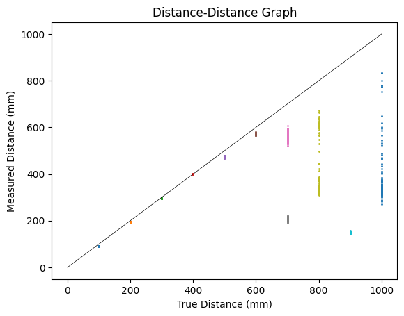
However, the Kalman filter is adjusted to work at terminal velocity, and really comes into play when the robot is close to the wall. Therefore, I only really care about this when the distance sensor is getting readings that are close to the wall, and therefore the variance is likely fairly low and likely does not change much as it gets closer and closer.
Based on this assumption, I placed the car around 300 millimeters away from my box and let the distance sensor absolutely go ham. It took 1024 samples, and with this, I calculated a variance of 1.2724571228027344. This will be used as my Sigma_z value.
Sigma_z = np.array([
[1.2724571228027344]
])
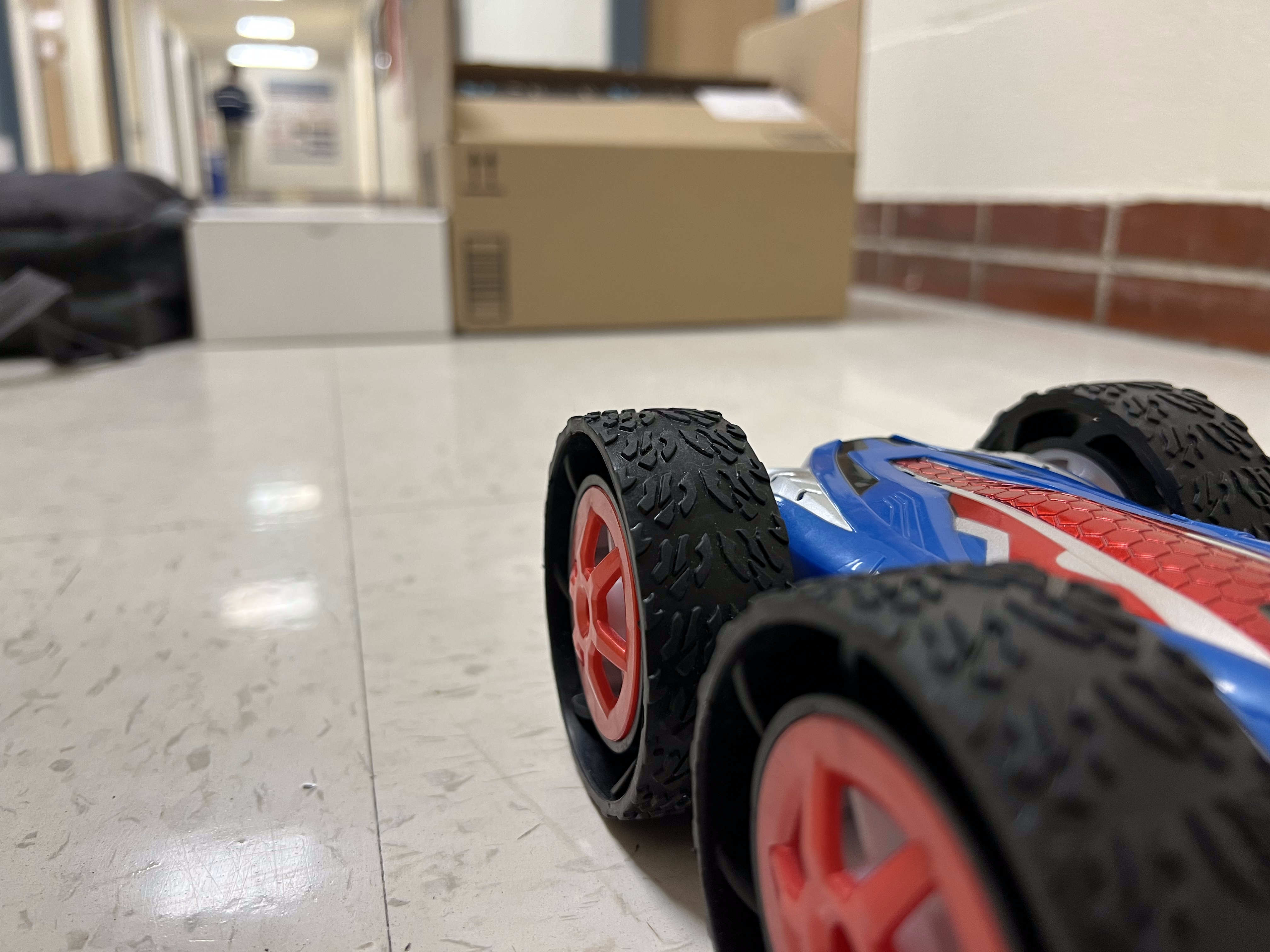
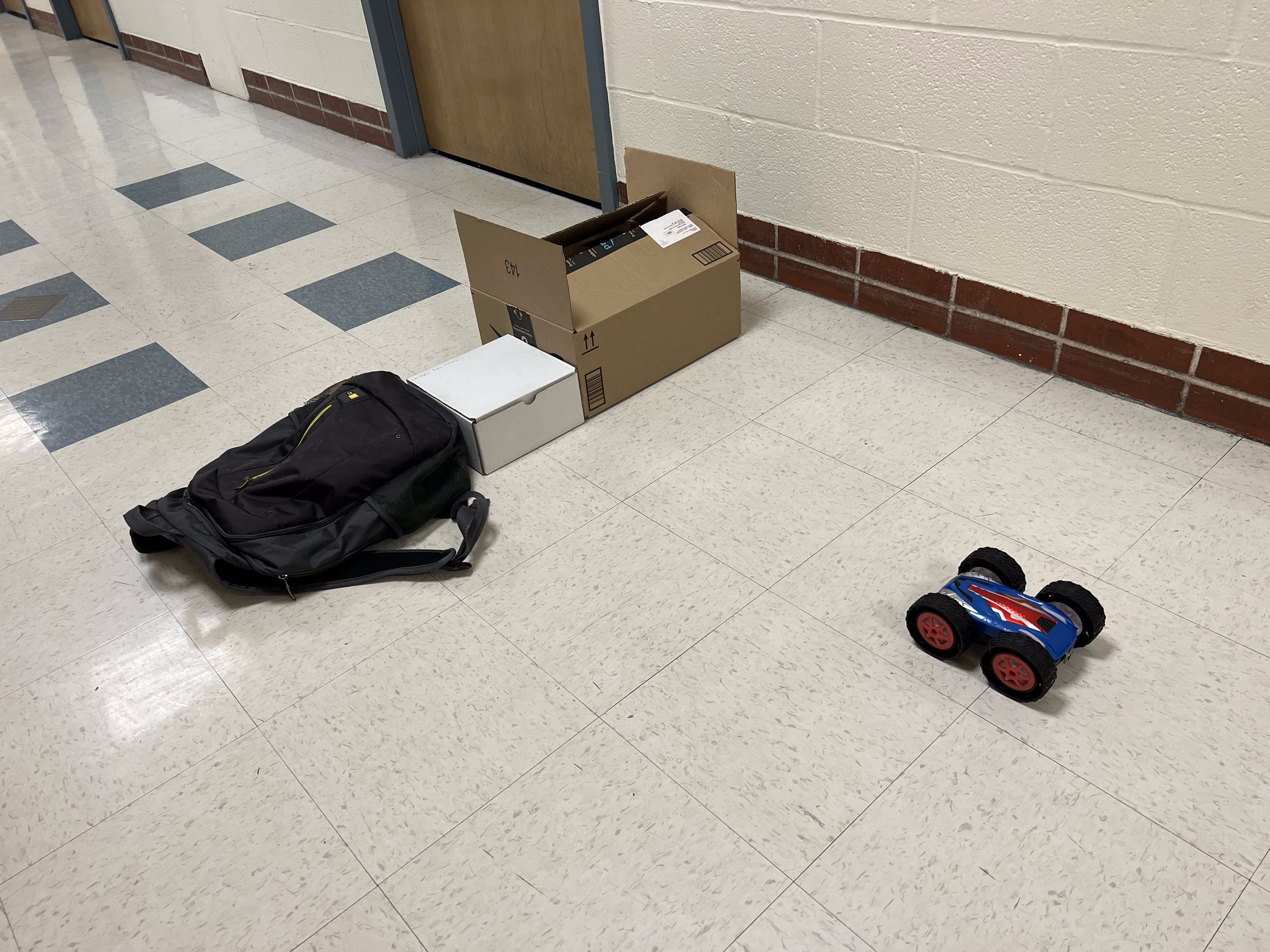
To estimate the drag, we need to get the robot up to full speed. It's hard to get to this point without risking many hours to fix a broken robot, so I tried to approach this a bit more cautiously. I used my box and my backpack as cushion, and I tried to get it to get to a point where it would mostly stay stright (my previous open-loop adjustments were for a speed of about 15%, not 75%), which took readjusting my pwm mappings. I also wanted to find a relatively good distance to space it. Too close it would never touch terminal velocity. Too far and it would veer off the straight path and I would lose control. But I also need it to be far enough to not only reach terminal, but maintain terminal velocity for a measurement or two so I could be fairly confident what terminal velocity actually is. However, data is gathered slow, so data resolution is pretty low. Which, funnily enough, is exactly what the Kalman filter is supposed to solve. Below is a slightly humorous picture of my robot facing off against the backpack/box wall, alongside a clearer image of my setup. The car, in reality, started much further back than this.
|
|
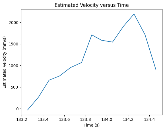
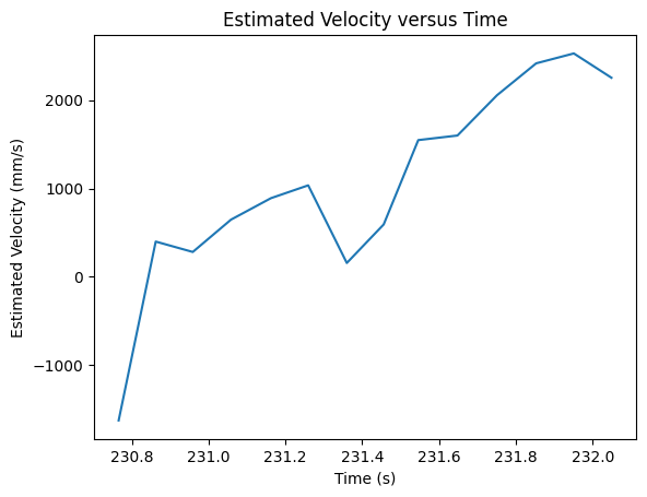
From this kind of setup came the first semi-successful attempt at gathering data, shown below.
Also, important to note is my code used to calculate this velocity.
# Calculate speed
velocity = []
print( [x[0] for x in front_distance] )
print( [t[1] for t in front_distance] )
for i in range( 1, len( front_distance ) ):
distance0, time0 = front_distance[i - 1]
distance1, time1 = front_distance[i]
# Negate velocity to be able to show it as a positive moving forward, instead of a negative closing of a gap
velocity.append( ( 1000*( distance0 - distance1 ) / ( time1 - time0 ), ( time1 + time0 ) / (2*1000) ) )
With the previous open-loop control, the right set of motors needed to be much stronger than the left. However, now my car is constantly veering left, so I definitely need to readjust and make the left relatively similar to the right.
The next successful attempt is shown below. It seemed to stop at the 1.5 second mark, which is what I set the cutoff of my PWM session. It also crashed into my backpack as it reached this point, but did not detect the closing of the distance because the sensor did not go off in time, so I do need to add a bit more in the way of distance so it can better reach terminal velocity.
Despite spending a lot of time trying to get this to work, I wasn't able to get a better sample, so I will just use the previous two, which are, though not perfect, honestly pretty fine.
The maximum velocity is about 2500 millimeters/second, from my second graph. My frist graph reached only around 2200 millimeters/second, but I can know not to use that because if it was faster in the second graph, it can at least reach that speed, meaning the first graph doesn't quite give the maximum. I will use this 2500 millimeters/second to estimate drag. We are told to use unity for steady-state input for now. Let's say force has units of kilogram*millimeters/second^2. Drag then has units of kilogram/second. With all of this, drag comes out to be 1/2500 kilograms/second, or about 0.0004 kilograms/second.
To estimate the mass, we first need to know how long it takes to get to 90% or so of terminal velocity from 0. 90% of terminal velocity is 2250 millimeters/second. To get to this velocity, estimated from the first graph, is about 1 second. Using the formula mass = ( -drag * time to 90% terminal velocity ) / ln( 1 - drag * 90% terminal velocity ), we get the mass is about 0.000173 kilograms. This is quite small, and will be scaled up once we start taking the fact that weused unity for the input into account. With this value for mass, we now have out A and B matricies. We also already had our C matrix. The following lines of code show how I derive those matricies in Python.
A = np.array([
[0,1],
[0,-d/m]
])
B = np.array([
[0],
[-1/m]
])
C = np.array([
[-1, 0]
])
This webpage was written in a mixture of during and after I implemented the Kalman filter, so it is liable to be a bit of a mess. But I want to take a nice little hindsight moment here to talk about a bug I faced. I was calling a matrix inverse, as given in the Kalman filter function provided. However, it was complaining about it being a zero-dimensional matrix instead of a two-by-two matrix. Rafi got it to be a one-dimensional matrix, or something of the sort. Ignacio then helped me see that I actually had a two-element array for C instead of a one-by-two matrix. And similar things occurred with some of my one-by-one matricies, which were just defined as single-element arrays. By not including an additional, necessary set of square brackets around my [-1,0] in my C definition, it was just an array and not a matrix.
We almost have everything we need. We just need to estimate what Sigma_u is. This is quite difficult, so I just chose a small and seemingly reasonable value of 10. I plan on adjusting it if it seems to be leading to unreasonable results (which, in hindsight, I did not need to adjust).
Sigma_u = np.array([
[10,0],
[0,10]
])
To implement the Kalman filter, I need to discretize the A and B matricies. This is important because we need to account for the time step, which is what this step does. I was honestly confused as to how to do this, until I looked closely at the slides and it soon instantly became clear what needed to be done. They outline a step-by-step derivation for the discretization, though we technically only need the last step of that derivation. This is the incredibly simple implementation in my Python code.
# Discretize the A and B matricies
Ad = np.eye(2) + dt*A
Bd = dt*B
Now, to get dt is a fairly straightforward task. It is supposed to be the difference between the sensor readings. Instead of choosing to vary that each time, I figured an average would do well. Of course, when I put this on the robot, this won't really be possible, but I can just use this value and trust that it will likely be good enough. After all, these are all just estimations on top of estimations. The following code shows how I calculated dt.
# Use the front_time readings to estimate the dt, sampling time
dt = 0
for i in range( 1, len( front_time ) ):
time0 = front_time[i - 1]
time1 = front_time[i]
# Accumulate all the time differences
dt += time1 - time0
# Average the time differences
dt /= len( front_distance ) - 1
# Scale to be seconds
dt /= 1000
This gave a value of 0.09871428571428571
This took me a bit longer to figure out than I'd like to admit and the inspiration likely came from one of the TA's websites, but this is literally just the initial sensor reading. For the run I was looking at, I had a sensor reading of 2455 millimeters.
# mu: The current estimate of the state vector (mean).
mu = np.array([
[front_distance[0]],
[0]
])
As many of these have been, this is a fairly strightforward value. I chose to make the control input a constant 0.75 across all iterations of the Kalman filter, as I did all my data gathering at 75% of max motor speed, according to my percentage to PWM value mapping function I made much earlier in the semester and modified as I mentioned in the drag section. This is made to be a one-by-one matrix.
u = np.array([
[0.75]
])
The final value we need is the Sigma matrix. This is one of those things that is hard to predict. Looking at Larry's website, I decided to borrow his values and adjust if needed. Which, similar to my other Sigma values, did not need adjustment.
# I took this from Larry's website
sigma = np.array([
[5**2,0],
[0,5**2]
])
After all of that estimation and gathering data and such, we are finally ready to run our Kalman filter. Here is the code I used to iterate through.
kf_distance_predictions = []
# Run the Kalman filter for each time step
for i in range( 0, len( front_time ) ):
mu, sigma = kf(mu, sigma, u, y[i])
kf_distance_predictions.append( mu[0] )
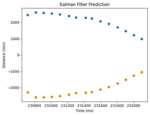
Oh no. The C matrix has its -1 value because we are operating under the assumption that our sensor readings are negative. Which they are. But I modify the values in my robot to make them positive, so I have to reflect that in the C matrix as well to remain consistent.
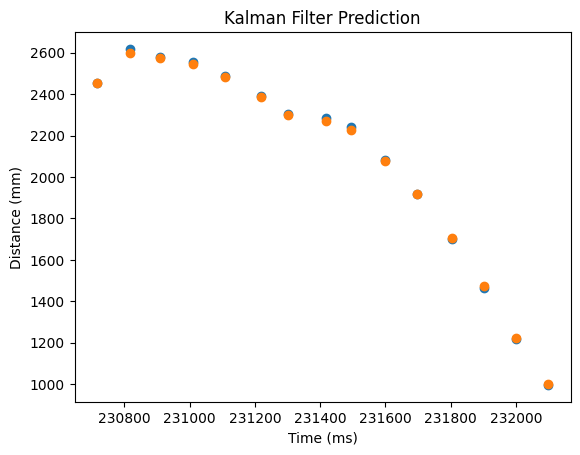
This is much better and shows that our Kalman filter now works as hoped. The Kalman filter is the orange plot, while the actual measured data from the car is the the blue plot.
This task now requires us to conditionally update the Kalman filter, or just simply use it to propagate forward a prediction. To do this, I will include a boolean called new_reading, which will be true whenever there is a new reading from the time of flight sensor and false whenver there is not a new reading from the time of flight sensor.
I use the following code for the new Kalman filter function, which was heavily influenced by Rafi's and Julian's code on their respective websites. It is essentially the same Kalman function, although it accounts for the case where there isn't new data, in which it uses mu_p and sigma_p as mu and sigma respectively.
# Kalman filter different frequency
def kf_df( mu, sigma, u, y, new_reading ):
mu_p = Ad.dot(mu) + Bd.dot(u)
sigma_p = Ad.dot(sigma.dot(Ad.transpose())) + Sigma_u
# If there is a new reading, act as before
if( new_reading ):
sigma_m = C.dot(sigma_p.dot(C.transpose())) + Sigma_z
kkf_gain = sigma_p.dot(C.transpose().dot(np.linalg.inv(sigma_m)))
y_m = y-C.dot(mu_p)
mu = mu_p + kkf_gain.dot(y_m)
sigma=(np.eye(2)-kkf_gain.dot(C)).dot(sigma_p)
# If there is no new reading, just use mu_p and sigma_p
else:
mu = mu_p
sigma= sigma_p
# Return the updated estimate of the state vector and estimate of the covariance matrix of the state vector
return mu,sigma
For the code that runs this function repeatedly so as to simulate the Kalman filter on the robot, I use the following code. This is heavily inspired by Julian's code on his website, but of course modified a little bit. I tried to explain it in depth in the code comments shown below, so I will spare you the duplicate explanation.
# dt for this is consistent because I am choosing to make it consistent for simulation's sake
# It would certainly vary on the robot.
# This is in units of seconds
dt = 0.01
# Rediscretize the A and B matricies with the established dt
Ad = np.eye(2) + dt*A
Bd = dt*B
# Empty the array to store our kalman filter predictions
kf_distance_predictions = []
# Create a variable to keep track of which sensor reading we are currently using
j = 0
# Create a variable to tell the Kalman filter (different frequency) function
new_reading = False
# Run the Kalman filter for each time step
# i starts at the first time of the simulation, which was the first time of the data gathering
# it goes to the last time of the data gathering (nothing stopping me from going at least a bit further, technically)
# It increments by dt scaled by 1000, to put it in units of milliseconds (and casted to int)
for i in range( front_time[0], front_time[len( front_time ) - 1], int(dt*1000) ):
# Check if there is a new reading (if i >= the front time of the next reading, then in
# simulation it is ready). Heavily inspired from Julian's code.
if( front_time[j + 1] <= i ):
# We are now on the new sensor reading
j += 1
new_reading = True
else:
# No new sensor reading yet
new_reading = False
# Call the kalman filter different frequency function, which takes into account new or no new readings
mu, sigma = kf_df(mu, sigma, u, y[j], new_reading)
# Append to the array we cleared earlier
kf_distance_predictions.append( mu[0] )
What this ends up looking like is the following. I changed a few parameters to have it behave a bit better, but I couldn't seem to fix the Kalman filter's prediction based on the first reading for some reason. I am not quite sure what causes it to behave this way, but my best guesses are that it is increasing while all other distances are decreasing, or just that it is the first and there's some edge case that I am missing. I changed Sigma_u's values of 10 to values of 25, and Sigma has its values of 25 go to 20.
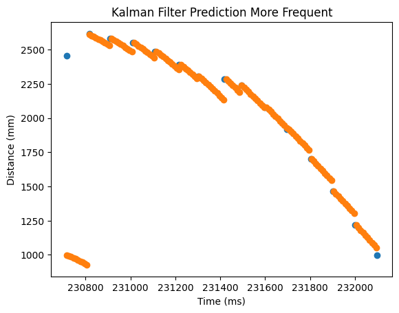
And with this, a working Kalman filter in simulation! How exciting : D
I plan on doing this! I haven't gotten to it yet but I would like to do it! : )
My front distance sensor at one point failed to connect. Killing the power (unplugging the battery and the USB-C connection) and turning it back on seemed to revitalize it. I'm not quite sure what caused such a thing, because usually restarting the Artemis seemed to not affect the distance sensors. My car, for some reason, moved backwards and then the sensor seems to have stopped working. Regluing the LED cover. You can find the list here.